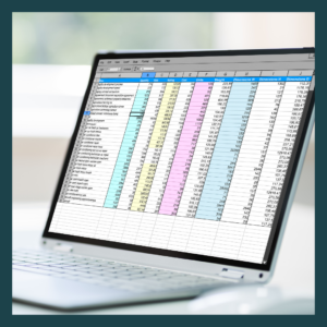
 Spreadsheet software such as Microsoft Excel offer immense value, but when data gets too complex, even common functions like filtering can become a hassle. This is especially true if you’re unfamiliar with Excel’s advanced features. However, with Microsoft Excel slicers, there’s a simple and visual way to filter data.
Understanding Excel slicers and how they improve data filtering
An Excel slicer is a powerful yet simple tool that helps users filter and interact with data based on selected criteria. It’s especially useful for drilling down into specific information within larger datasets. Once a slicer is set up in a worksheet, it allows users to quickly filter data by clicking buttons that correspond to particular groups of information. This makes it easy to isolate key insights without needing to scroll through long rows of data.
Excel already offers built-in filtering options for both tables and PivotTables, but these can sometimes feel cumbersome, particularly with larger datasets. Slicers provide a more intuitive, visually appealing way to filter information, streamlining the process.
Slicers are most commonly used with tables and PivotTables, enabling users to create multiple slicers for the same dataset. This allows viewers to easily see which subsets of data are being filtered and adjust the view according to their needs. With just a few clicks on the slicer buttons, specific datasets can be highlighted, offering a clearer focus.
In addition to tables and PivotTables, slicers can also be applied to charts, further enhancing the ability to interact with and filter graphical data representations. This versatility makes slicers a go-to tool for anyone looking to manage complex datasets more effectively.
How to create and customize slicers in Excel
Before you can start using slicers in Excel, you should first organize your data into a table. Begin by selecting the entire dataset you want to work with. Then, navigate to the Ribbon toolbar at the top of the screen, select Insert, and choose Table. Ensure the option for “My table has headers” is checked in the popup window before clicking OK.
Once your data is formatted as a table, you can easily add slicers. Simply click on any cell within the table, go back to the Ribbon, and select Insert > Slicer. In the dialog box that appears, you will be prompted to select which fields (based on your headers) you want to use as slicers. You can select one or multiple fields, depending on what data you’d like to filter. Once you’ve selected the fields, click OK to generate the slicers.
The slicers will appear on your worksheet, and each slicer will contain buttons that correspond to the data in the chosen fields. You can rearrange the slicers on your sheet for clarity and ease of use, ensuring they are neatly spread out and easy to read.
You can also enhance the slicers by changing their appearance. Excel allows you to customize the color of each slicer for visual distinction or to match the overall style of your sheet. To change the slicer’s color, click on the slicer you want to modify, go to the Slicer tab on the Ribbon, and choose a new color from the available options in the gallery.
Finally, repeat the color customization process for each of your slicers to keep them visually organized and user-friendly.
Beyond slicers, there are countless other features in Excel and the Microsoft Office suite that can help streamline your workflow. If you’re interested in exploring more of these functions or need assistance in setting up the best Office tools for your business, don’t hesitate to contact our team. We’re here to help you unlock the full potential of Microsoft Office.


